The Toolbox 🧰 🦀

Aug, 10th 2026: A third off the run time of the partitioner

Chipper takes a road network and cuts it into cells. It picks a cut with the Inertial Flow method, splits the graph along that cut, and repeats on both halves until the pieces are small enough. On the road network of the USA that means about eighteen useful levels of recursion and roughly 365,000 cells at the end.

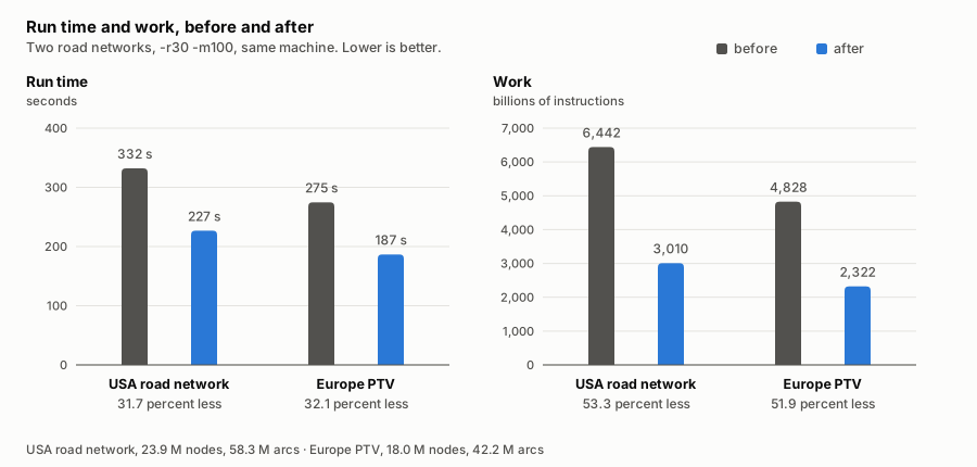
The tool worked. It was also doing about twice as much work as it needed to. Taking that work out cut the run time by about a third, from 332 seconds to 227 on the USA network and from 275 to 187 on Europe. This post walks through where the work was, why removing half of it bought only a third of the time, and which two attempts looked promising and then failed to pay off.

That is the output after nine levels, drawn from the convex hulls the scaffold tool writes as GeoJSON. The long thin shapes are cells whose nodes wrap around water, so their hull spans the gap.

Measuring first

Run time is what matters and it is also the hardest thing to measure. The same binary on the same input does not take the same time twice. Every comparison here was therefore measured more than once, with the before and after runs interleaved, so that whatever else the workstation is doing cannot settle on one side of it. Instructions retired, which /usr/bin/time -l reports on macOS, is far steadier from run to run.

So the two numbers do different jobs here. Wall clock says whether the tool got faster. Instructions retired says whether a particular change was the reason, and it is what the individual steps below are quoted in. The two do not move by the same amount, which gets its own section further down.

Two inputs were used, both with -r30 -m100, the invocation from the README. The USA road network from the 9th DIMACS challenge has 23.9 million nodes and 58.3 million arcs. The europe.ptv instance has 18.0 million nodes and 42.2 million arcs.

A change that makes the tool faster and the partition worse is not a win, so every step was also checked by hashing the full assignment and counting how many edges the final partition cuts.

Where the time went

A sampling profiler answers this, but the first answer is useless. With link time optimization on, almost everything is inlined into one symbol, and the profile reports 69 percent of the time in sub_step without saying what sub_step was doing. Marking four functions #[inline(never)] for one throwaway build gives the real picture:

function	share of run time
Dinic::bfs	26.9 percent
sub_step itself	24.4 percent
sorting node ids	11.3 percent
threads waiting	7.9 percent
Dinic::from_edge_list	6.7 percent
Dinic::dfs	2.4 percent

An earlier profile of the untouched code put a comparison sort inside from_edge_list at about 24 percent on its own. That is where this started.

Building the flow graph without sorting it

The max flow solver needs a residual graph, which holds a reverse arc of zero capacity for every input arc so that flow can be pushed back later. The old code built it by copying the entire edge list onto itself, flipping the copy, sorting all of it by source and target, and merging the duplicates back together.

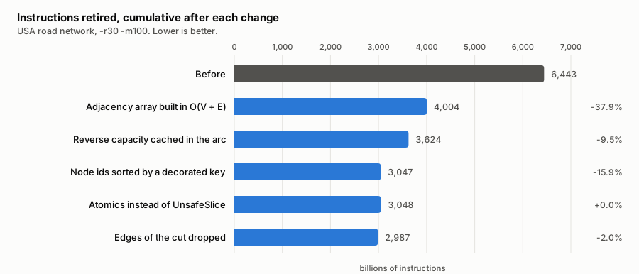
Sorting is the expensive part and it is not needed. The node ids of a cell are already numbered densely from zero, which is what a counting sort is for. Count how many arcs each node owns, turn the counts into offsets with a prefix sum, and scatter the arcs into their blocks. That builds the adjacency array directly in linear time. Only the blocks themselves still get sorted, and a block in a road network holds about five arcs.

The result was 37.9 percent fewer instructions for the whole run, and the partition it produced was identical bit for bit.

The lookup that dominated the BFS

With the sort gone, the breadth first search became the most expensive part of the program. Its inner loop walks the arcs of a node, and for each arc it needs to know the capacity of the arc pointing the other way. It found that arc by scanning the adjacency block of the head until the target matched.

The obvious fix is a table holding the id of the reverse arc for every arc, built once with the graph. That was tried first, and it cut instructions by 4 percent while making the program slower. Filling the table costs a binary search per arc and those searches jump all over the edge array, so the instruction count went down as the cache behaviour got worse. This is the case that counting instructions alone would have got wrong.

The version that worked stores the capacity of the reverse arc inside each arc instead of its id, so the breadth first search needs no lookup at all. The value it wants is already in the record it is reading. Two details make this free rather than merely cheap. It can be filled in during the scatter, since an input arc contributes its capacity to the forward arc and to the reverse capacity of its partner. And the adjacency array entry had four bytes of padding sitting unused next to the node id.

The depth first search does still have to find the partner arc, because it keeps both halves of a pair in step when it pushes flow. A binary search serves, since the targets inside a block are sorted, and it runs once per arc on an augmenting path rather than once per step of the search. This was worth 9.5 percent of the remaining instructions and 13 percent of the CPU time, again with a bit identical partition.

Sorting node ids without chasing pointers

Inertial Flow sorts the nodes of a cell by their position projected onto one of four axes. The code did that with sort_unstable_by_key, where the key function reads the coordinate of the node. That is convenient, and it means every comparison performs a random read into a coordinate array of 24 million entries. A sort makes on the order of n log n comparisons to compute a value that only takes n evaluations to precompute.

Attaching the projected value to each id once and sorting the pairs removed 16 percent of the instructions. This is the one change that alters the result, because ties between nodes with the same projected position now break differently. The partition it produces cuts 52 fewer edges out of 2.7 million, so the tie breaking is not worse.

Removing the unsafe code, for free

The partitioner wrote its cell ids through a helper called UnsafeSlice, which hands out mutable references from a shared one. The reasoning behind it was sound. Cells are disjoint, so no two threads ever write the same entry. The helper itself was not sound, because it was Sync and its read method was safe, so two threads could take a shared reference and a mutable reference to the same index without writing unsafe anywhere.

Relaxed atomics make the same claim the helper was making, but they differ in what happens when the claim turns out to be wrong. UnsafeSlice states it as a promise to the compiler, and a broken promise there is undefined behaviour, which means the compiler is entitled to generate code on the assumption that it cannot happen. An atomic makes the access legal whether the claim holds or not. A mistake then costs a wrong cell id instead of a program optimised on a false premise. For an invariant that no tool checks, that is the better failure mode.

Which ordering to ask for is the interesting part, and it is where the shape of the program pays off. Relaxed promises nothing about any other memory. It only guarantees that the access itself is not a data race and that repeated reads of one location see a coherent sequence of values. That is enough here, for two separate reasons. Within a level, a thread only ever reads entries it wrote itself, because once the edges of the cut are dropped both endpoints of every edge belong to the cell being split. Between levels, the parallel loop joins, and that join is what makes the writes of one level visible to the next.

The ordering was already there, supplied by the fork and join of the parallel iterator, so reaching for Acquire and Release out of caution would have paid for it twice. That is the useful part of having to name an ordering. It forces the question of which happens-before edges the code actually depends on, and here the answer was none that the atomics had to provide.

On x86-64 and on AArch64 a relaxed load and a relaxed store compile to the same instructions as a plain load and a plain store, so none of this costs anything to execute. The measurement agrees. The difference was 0.03 percent, which is noise, and the partition came out identical. The partitioner now contains no unsafe at all, and the helper, which had no user left in the crate, was deleted in #543.

Dropping the edges of the cut

When a cell splits, its edges have to be handed down to the two halves. The old code decided by the tail of each edge only. An edge running from the left half to the right half therefore stayed with the left half, and at the next level its head was renumbered into the flow graph as an extra node.

Such a node can never carry flow. Its only outgoing arc is a reverse arc with zero capacity, so the search reaches it and stops. It just made every flow graph a bit bigger than it needed to be, and the effect grows as cells get smaller and their boundary grows relative to their interior. Checking both endpoints and dropping the edges of the cut removed another 2 percent of the instructions.

What did not work

About a quarter of the machine sits idle during a run. The obvious suspect was the barrier at the end of each level, where every thread waits for the largest cell of that level. Rewriting the driver as a recursion, with the two halves of a cell handed to a work stealing fork, removes that barrier entirely.

It made things slower. Wall clock went from 194 seconds to 203 and the average number of busy cores dropped from 6.0 to 5.7. The partition was identical, so this was purely a scheduling change, and the schedule got worse.

Two profiles explain it. Idle time is 54.6 percent during the first levels of the recursion and only 7.9 percent in the middle of the run. The threads are not waiting at the barrier. They are waiting at the top of the tree, where there is one cell to work on and the algorithm offers four independent tasks, one per axis. Eight cores cannot be kept busy by four tasks however they are scheduled, and fixing that needs parallelism inside a single cell.

Two bugs found on the way

Reading the code closely also turned up two defects that had nothing to do with speed. A node that no edge of its cell touches was dropped from both halves of a split, so it never descended again and kept a cell id from a level higher up while every other node ended at the bottom of the hierarchy. At the root that affects any node no edge of the whole graph touches, and isolated nodes are common in extracted road networks. A cell that none of the four axes could cut had the same problem for all of its nodes. Both now descend properly, and a cell with no edges reports an error instead of handing an empty graph to the max flow solver.

Why half the work is not half the time

The instruction count fell by 53 percent on the USA network and the run time by 32 percent. That gap is not a rounding error and it is worth taking apart, because a program is not a machine that executes a fixed number of instructions per second.

Dividing instructions by CPU time gives 3.40 billion per second before and 2.57 billion after. The code that remains executes fewer instructions per second than the code that was removed, which is what you would expect from what was removed. A comparison sort and a linear scan are both instruction dense and reasonably kind to the cache. What is left is dominated by a breadth first search over an adjacency array of tens of millions of arcs, and that search spends much of its time waiting for memory rather than executing anything.

Dividing CPU time by wall clock gives 5.7 of 8 cores busy before and 5.2 after. The idle fraction grew too, for the reason in the section above. A shorter run spends proportionally more of itself at the top of the recursion, where there is one cell to split and only four tasks to hand out.

Neither effect is a reason to stop counting instructions. They are the reason to count them and the clock separately.

Where it ended up

metric	USA before	USA after	Europe before	Europe after
wall clock	332.1 s	226.7 s	274.7 s	186.6 s
CPU time	1892.2 s	1171.3 s	1572.0 s	1028.2 s
instructions retired	6,441.8 G	3,009.7 G	4,827.5 G	2,322.0 G
peak memory	10.26 GB	11.02 GB	7.37 GB	7.05 GB
cut edges	2,667,702	2,667,614	1,959,596	1,959,521

Run time falls by just under a third on both networks while the instruction count falls by about half, and the cut gets slightly smaller on both. Peak memory is a wash. It went up 7 percent on the one network and down 4 percent on the other, and repeated runs of the unchanged binary already spread over 11 percent on the USA input, so neither direction is worth reading as a result.

The work is in #542.

Jun, 13th 2022: Fixing a scalability issue

The recursive bi-partitioning exhibited a flaw in the amount of memory it allocated. The following graph shows how the performance regressed for levels greater or equal to 8. The graph shoots up exponentially. The issue was fixed in #89 by making sure that the per sub-graph memory allocation is independent of the overall graph size but only depends the size of the subgraph. Note that the speedup of the fixed version is super-liner.